Solid primitives by domain mapping

The mapper.jl file contains the implementation of several parametric primitives, including curves, surfaces and solids embedded in either 2D or 3D.

The constructive approach is common to all methods. It consists in generating a simplicial or cuboidal decomposition of a simple geometrical domain in u,v or u,v,w parametric space. Then a change of coordinates, e.g. from Cartesian to polar or cylindrical coordinates, is applied to the vertices of the cellular complex decomposing the domain.

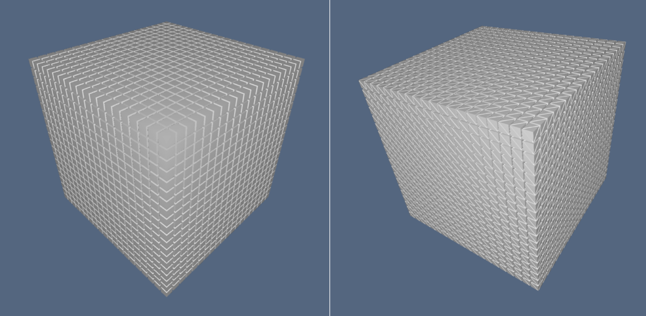
Figure 1: Cellular 3-complexes, slightly exploded: (a) cuboidal mesh; (b) simplicial mesh.

So, the mapped domain produces a curved manifold in 2D or 3D space. To obtain a closed curved surface, i.e. a manifold-without-boundary, as in the case of a 2-sphere in 3D, or of the toroidal surface in 3D, a suitable identification of coincident mapped points is performed.

Basics of LAR models

A very simple LAR model is a 2D square with a vertex on the origin:

julia> square=([[0.; 0] [0; 1] [1; 0] [1; 1]], [[1,2,3,4]], [[1,2], [1,3], [2,4], [3,4]])
([0.0 0.0 1.0 1.0; 0.0 1.0 0.0 1.0], Array{Int64,1}[[1, 2, 3, 4]], Array{Int64,1}[[1, 2],
[1, 3], [2, 4], [3, 4]])

Conventional names for the arrays of vertices, faces and edges:

julia> V,FV,EV = square
([0.0 0.0 1.0 1.0; 0.0 1.0 0.0 1.0], Array{Int64,1}[[1, 2, 3, 4]], Array{Int64,1}[[1, 2],
[1, 3], [2, 4], [3, 4]])

V may be either of type Array{Float64,2} or Array{Int64,2}

julia> Lar = LinearAlgebraicRepresentation

julia> V::Lar.Points
2×4 Array{Float64,2}:
 0.0  0.0  1.0  1.0
 0.0  1.0  0.0  1.0

The arrays containing the $p$-dimensional ($2\leq p\leq d$) cells of a $d$-complex must be of type Array{Array{Int64,1},1}, where each element contains the unordered array of indices of vertices on the boundary of the cell:

julia> EV::Lar.Cells
4-element Array{Array{Int64,1},1}:
 [1, 2]
 [1, 3]
 [2, 4]
 [3, 4]

Cuboidal and simplicial grids

LinearAlgebraicRepresentation, as its ancestor geometric language PLaSM and its father library pyplasm aims to be multidimensional. Hence some functions generate geometric models of varying dimensions. Important examples are cuboidGrid and simplexGrid, whose unique parameter is the shape of the generated mesh, i.e. the number of $d$-dimensional cells in each dimension, with d = length(shape). The vertices of the mesh stay on the integer grid of suitable dimension and size.

julia> shape = [1,1,1]

julia> Lar.cuboidGrid(shape)
([0.0 0.0 … 1.0 1.0; 0.0 0.0 … 1.0 1.0; 0.0 1.0 … 0.0 1.0], 
Array{Int64,1}[[1, 2, 3, 4, 5, 6, 7, 8]])

Hence we have, for single-cell 1-, 2-, 3-, and 4-dimensional LAR models:

julia> Lar.cuboidGrid([1])
([0.0 1.0], Array{Int64,1}[[1, 2]])

julia> Lar.cuboidGrid([1,1])
([0.0 0.0 1.0 1.0; 0.0 1.0 0.0 1.0], Array{Int64,1}[[1, 2, 3, 4]])

julia> Lar.cuboidGrid([1,1,1])
([0.0 0.0 … 1.0 1.0; 0.0 0.0 … 1.0 1.0; 0.0 1.0 … 0.0 1.0], 
Array{Int64,1}[[1, 2, 3, 4, 5, 6, 7, 8]])

julia> Lar.cuboidGrid([1,1,1,1])
([0.0 0.0 … 1.0 1.0; 0.0 0.0 … 1.0 1.0; 0.0 0.0 … 1.0 1.0; 0.0 1.0 … 0.0 1.0],
Array{Int64,1}[[1, 2, 3, 4, 5, 6, 7, 8, 9, 10, 11, 12, 13, 14, 15, 16]])

Two examples follows for a $20\times 20$ mesh in 2D, and a $20\times 20\times 20$ mesh in 3D. Of course, their highest dimensional cells (quads and hexs) have 4 and 8 vertices, respectively.

julia> Lar.cuboidGrid([20,20])
([0.0 0.0 … 20.0 20.0; 0.0 1.0 … 19.0 20.0], Array{Int64,1}[[1, 2, 22, 23], [2, 3, 23,
24], [3, 4, 24, 25], [4, 5, 25, 26], [5, 6, 26, 27], [6, 7, 27, 28], [7, 8, 28, 29], [8,
9, 29, 30], [9, 10, 30, 31]  …  [415, 416, 436, 437], [416, 417, 437, 438], [417, 418,
438, 439], [418, 419, 439, 440], [419, 420, 440, 441]])

julia> Lar.cuboidGrid([20,20,20])
([0.0 0.0 … 20.0 20.0; 0.0 0.0 … 20.0 20.0; 0.0 1.0 … 19.0 20.0], Array{Int64,1}[[1, 2,
22, 23, 442, 443, 463, 464], [2, 3, 23, 24, 443, 444, 464, 465], [3, 4, 24, 25, 444, 445,
465, 466]  …   [8797, 8798, 8818, 8819, 9238, 9239, 9259, 9260], [8798, 8799, 8819, 8820,
9239, 9240, 9260, 9261]])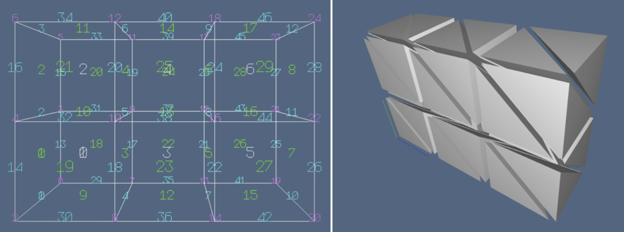

Figure 2: Cellular 3-complexes: (a) cuboidal mesh, with 0-, 1-, 2-, and 3-cells numbered with different colors; (b) exploded simplicial mesh, with 6 tetrahedra (3-cells) per mesh cube.

Similarly, you can generate a multidimensional mesh of $d$-simplexes ($d=1,2,3,\dots$) with the simplexGrid function, having as single parameter the (cuboidal) shape of the mesh.

Let us generate $d$ (increasing in dimension) simplicial complexes partitioning a single hypercube $[0,1]^d$:

julia> Lar.simplexGrid([1]) # one segment in [0,1] 
# output
([0.0 1.0], Array{Int64,1}[[1, 2]])

julia> Lar.simplexGrid([1,1]) # two triangles in [0,1]^2 
# output
([0.0 1.0 0.0 1.0; 0.0 0.0 1.0 1.0], Array{Int64,1}[[1, 2, 3], [2, 3, 4]])

julia> Lar.simplexGrid([1,1,1])  # six tetrahedra in [0,1]^3 
# output
([0.0 1.0 … 0.0 1.0; 0.0 0.0 … 1.0 1.0; 0.0 0.0 … 1.0 1.0], Array{Int64,1}[[1, 2, 3, 5],
[2, 3, 5, 6], [3, 5, 6, 7], [2, 3, 4, 6], [3, 4, 6, 7], [4, 6, 7, 8]])

julia> Lar.simplexGrid([1,1,1,1])  # 24 pentatopes in [0,1]^4 
# output
([0.0 1.0 … 0.0 1.0; 0.0 0.0 … 1.0 1.0; 0.0 0.0 … 1.0 1.0; 0.0 0.0 … 1.0 1.0],
Array{Int64,1}[[1, 2, 3, 5, 9], [2, 3, 5, 9, 10], [3, 5, 9, 10, 11], [5, 9, 10, 11, 13],
[2, 3, 5, 6, 10]  …  [4, 6, 7, 11, 12], [6, 7, 11, 12, 14], [7, 11, 12, 14, 15], [4, 6, 7,
8, 12], [6, 7, 8, 12, 14], [7, 8, 12, 14, 15], [8, 12, 14, 15, 16]])

Then look at the simplicial partition (3D triangulation) of the domain $[0,20]\times[0,20]\times[0,20] \subset \mathbf{R}^3$ shown in Figure 1b, and generated by the Julia expression below:

julia> Lar.simplexGrid([20,20,20]) 
# output
([0.0 1.0 … 19.0 20.0; 0.0 0.0 … 20.0 20.0], Array{Int64,1}[[1, 2, 22], [2, 22, 23], [2,
3, 23], [3, 23, 24], [3, 4, 24], [4, 24, 25], [4, 5, 25], [5, 25, 26], [5, 6, 26], [6, 26,
27]  …  [415, 416, 436], [416, 436, 437], [416, 417, 437], [417, 437, 438], [417, 418,
438], [418, 438, 439], [418, 419, 439], [419, 439, 440], [419, 420, 440], [420, 440,
441]])

List of currently available primitives

The mapper module aims to provide the tools needed to apply both dimension-independent affine transformations and general simplicial maps to geometric objects and assemblies developed within the LAR scheme. A large number of surfaces and primitives solids are definable using the map function and the local parametrization.

Curves

Primitive one-dimensional objects:

circle - Circle centered in the origin
helix - Helix curve about the z axis

Surfaces

Figure 3: Cellular 1- and 2-complexes: (a) 2D unit circle; (b) spiral curve embedded in 3D; (c) 2D unit disk; (3) spiraloid surface in 3D.

Primitive two-dimensional objects:

disk - Disk centered in the origin
helicoid - Helicoid about the z axis
ring - Ring centered in the origin
cylinder - Cylinder surface with z axis
sphere - Spherical surface of given radius
toroidal - Toroidal surface of given radiuses
crown - Half-toroidal surface of given radiuses

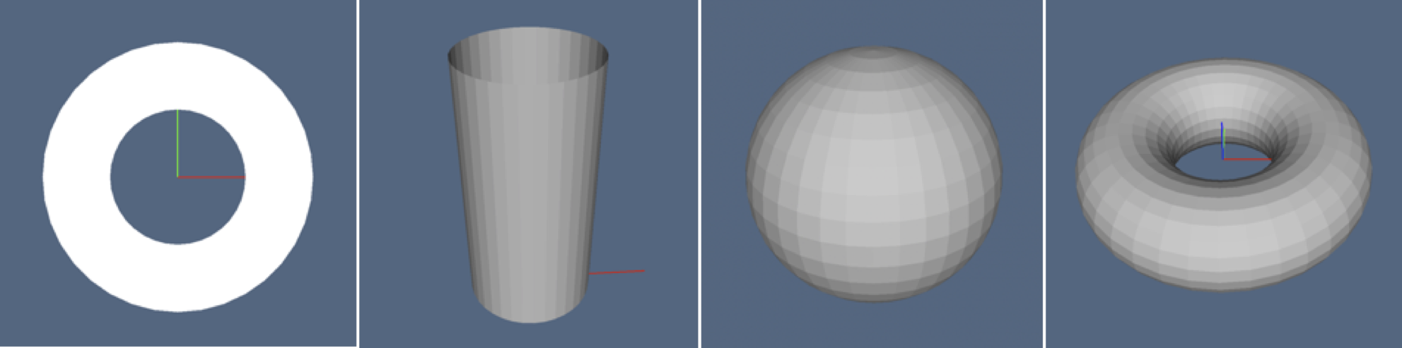
Figure 4: Cellular 2- and 3-complexes: (a) 2D disk; (b) cylinder surface in 3D; (c) 2-sphere surface in 3D; (3) toroidal surface in 3D.

Solids

Primitive three-dimensional objects:

cuboid - Solid cuboid of given extreme vectors
ball - Solid Sphere of given radius
rod - Solid cylinder of given radius and height
hollowCyl - Hollow cylinder of given radiuses and height
hollowBall - Hollow sphere of given radiuses
torus - Solid torus of given radiuses
pizza - Solid pizza of given radiuses

Figure 5: Cellular complexes: (a) 1-skeleton of 3D cube; (b) assembly of cell complexes of mixed dimensions; (c) 3-mesh of portion of hollow solid cylinder; (d) 3-mesh of a portion of hollow solid torus.

Implementation

The coding of the generating functions for the various geometric primitives follows the below guidelines:

* Higher level function interface. Every generating function is of type $fun: parms_1 \to (parms_2 \to results),$ with $parms_1=p_1\times p_2\times cdots \times p_m$ and $parms_2=q_1\times q_2\times cdots \times q_n$. The $p_i$ parameters concern the specification of the coordinate functions of the mapping. The $q_j$ parameters ($1\leq j\leq n\in\{1,2,3\}$) affect the discretization of mapping domain.

* Simplicial or cuboidal decomposition. Discretization primitives simplexGrid() or cuboidGrid() are used for the two cases. Both primitives are dimension-independent, i.e. may decompose 1D, 2D, 3D,..., nD domains, depending only on the array shape of the generated cellular complex. The complex is generated in LAR format (vertices,cells), where vertices have integer coordinates.

* Coordinate functions. Are applied to the integer vertices, so producing their mapped instances and store them in a Array{Array{Int64,1},1}

* Complex simplification. Finally, the geometrically coincident vertices are identified, the generated cells are translated to the new vertex indices, and cells are simplified from multiple identical indices. This may induce the sewing of domain boundaries according to expected topology of the curved manifold and/or the reduction of independent vertices in cells of the complex.

Main Interface

Curve primitives

LinearAlgebraicRepresentation.circle — Function

circle(radius=1.; angle=2*pi)(shape=36)

Compute an approximation of the circunference curve in 2D, centered on the origin.

With default values, i.e. circle()(), return the whole circonference of unit radius, approximated with a shape=36 number of 1-cells.

Example

julia> W,CW = Lar.circle()();

julia> GL.VIEW([
	GL.GLLines(W, CW, GL.COLORS[12]),
	GL.GLFrame
]);

source

LinearAlgebraicRepresentation.helix — Function

helix(radius=1., pitch=1., nturns=2)(shape=36*nturns)

Compute the approximate elix curve in three-dimensional space, with basis on $z=0$ plane and centered around the $z$ axis. The pitch of a helix is the height of one complete helix turn, measured parallel to the axis of the helix.

Example

julia> V, CV = Lar.helix(.1, .1, 10)()
([0.1 0.0984808 … 0.0984808 0.1; 0.0 0.0173648 … -0.0173648 0.0; 0.0 0.0027778 … 0.997222 1.0], Array{Int64,1}[[1, 2], [2, 3], [3, 4], [4, 5], [5, 6], [6, 7], [7, 8], [8, 9], [9, 10], [10, 11]  …  [351, 352], [352, 353], [353, 354], [354, 355], [355, 356], [356, 357], [357, 358], [358, 359], [359, 360], [360, 361]])

julia> GL.VIEW([
	GL.GLLines(V, CV, GL.COLORS[12]),
	GL.GLFrame
]);

source

Surface primitives

LinearAlgebraicRepresentation.disk — Function

disk(radius=1., angle=2*pi)(shape=[36, 1])

Compute the cellular complex approximating a circular sector of 2D disk centered on the origin. In geometry, a disk is the region in a plane bounded by a circle. The shape array provides the number of approximating 2-cells.

Example

julia> GL.VIEW([
	GL.GLGrid( Lar.disk()()..., GL.COLORS[1],1 ),
	GL.GLFrame
]);

source

LinearAlgebraicRepresentation.helicoid — Function

helicoid(R=1., r=0.5, pitch=1., nturns=2)(shape=[36*nturns, 2])

Compute an approximation of the helicoid surface in 3D, with basis on $z=0$ plane and centered around the $z$ axis.

Example

julia> GL.VIEW([
	GL.GLGrid( Lar.helicoid()()..., GL.COLORS[1],1 ),
	GL.GLFrame
]);

source

LinearAlgebraicRepresentation.ring — Function

ring(r=1., R=2., angle=2*pi)(shape=[36, 1])

Compute the cellular 2-complex approximating a (possibly full) sector of a non-contractible disk. R and r are the external and the internal radiuses, respectively.

Example

julia> GL.VIEW([
	GL.GLGrid( Lar.ring()()..., GL.COLORS[1],1 ),
	GL.GLFrame
]);

source

LinearAlgebraicRepresentation.cylinder — Function

cylinder(radius=.5, height=2., angle=2*pi)(shape=[36, 1])

Compute a cellular 2-complex, approximation of a right circular cylindrical surface in 3D. The open surface has basis on $z=0$ plane and is centered around the $z$ axis.

Example

julia> GL.VIEW([
	GL.GLGrid( Lar.cylinder()()..., GL.COLORS[1],1 ),
	GL.GLFrame
]);

source

Missing docstring.

Missing docstring for Lar.sphere. Check Documenter's build log for details.

LinearAlgebraicRepresentation.toroidal — Function

toroidal(r=1., R=2., angle1=2*pi, angle2=2*pi)(shape=[24, 36])

Compute a cellular 2-complex, approximation of the two-dimensional surface, embedded in a three-dimensional Euclidean space. Toroidal is a closed surface having genus one, and therefore possessing a single "hole". It can be constructed from a rectangle by gluing both pairs of opposite edges together with no twists.

Example

julia> GL.VIEW([
	GL.GLGrid( Lar.toroidal()()..., GL.COLORS[1],0.75 ),
	GL.GLFrame
]);

source

Solid primitives

LinearAlgebraicRepresentation.cuboid — Function

cuboid(maxpoint::Array, full=false, minpoint::Array=zeros(length(maxpoint)))

Return a $d$-dimensional cube, where $d$ is the common length of arrays minpoint and maxpoint. If flag=true the cells of all dimensions (between 1 and $d$) are generated.

julia> cuboid([-0.5, -0.5])
([0.0 0.0 -0.5 -0.5; 0.0 -0.5 0.0 -0.5], Array{Int64,1}[[1, 2, 3, 4]])

julia> cuboid([-0.5, -0.5, 0], true)
([0.0 0.0 … -0.5 -0.5; 0.0 0.0 … -0.5 -0.5; 0.0 0.0 … 0.0 0.0],
Array{Array{Int64,1},1}[Array{Int64,1}[[1], [2], [3], [4], [5], [6], [7], [8]],
Array{Int64,1}[[1, 2], [3, 4], [5, 6], [7, 8], [1, 3], [2, 4], [5, 7], [6, 8], [1, 5], [2,
6], [3, 7], [4, 8]], Array{Int64,1}[[1, 2, 3, 4], [5, 6, 7, 8], [1, 2, 5, 6], [3, 4, 7,
8], [1, 3, 5, 7], [2, 4, 6, 8]], Array{Int64,1}[[1, 2, 3, 4, 5, 6, 7, 8]]])

julia> V, (VV, EV, FV, CV) = Lar.cuboid([1,1,1], true);

julia> assembly = Lar.Struct([ (V, CV), Lar.t(1.5,0,0), (V, CV) ])

julia> GL.VIEW([
	GL.GLPol( Lar.struct2lar(assembly)..., GL.COLORS[1],0.75 ),
	GL.GLFrame ]);

source

LinearAlgebraicRepresentation.ball — Function

ball(radius=1, angle1=pi, angle2=2*pi)(shape=[18, 36,4])

Generate a cell decomposition of a solid 3-sphere in $R^3$. The variable shape provides the domain decomposition. Empty cells are removed after the Cartesian -> Polar coordinate mapping.

Example

julia> GL.VIEW([
	GL.GLPol( Lar.ball()()..., GL.COLORS[1],0.5 ),
	GL.GLFrame ]);

source

LinearAlgebraicRepresentation.hollowCyl — Function

hollowCyl(r=1., R=2., height=6., angle=2*pi)(shape=[36, 1, 1])

Compute the cellular 3-complex approximating a solid cylinder with a internal axial hole. The model is meshed with cubical 3-cells.

Example

julia> GL.VIEW([
 	GL.GLPol( Lar.hollowCyl()()..., GL.COLORS[1],0.5 ),
 	GL.GLFrame ]);

source

LinearAlgebraicRepresentation.hollowBall — Function

hollowBall(r=1., R=2., angle1=pi, angle2=2*pi)(shape=[36, 1, 1])

Compute the cellular 3-complex approximating a 3-sphere. The model is meshed with cubical 3-cells, where the mesh has default decomposition size [24, 36, 8].

Example

julia> V, CV = Lar.hollowBall(1, 2, pi/2, pi/2)([6, 12, 4]);

julia> GL.VIEW([
 	GL.GLPol( V, CV, GL.COLORS[1],0.5 ),
 	GL.GLFrame ]);
...

source

LinearAlgebraicRepresentation.torus — Function

torus(r=1., R=2., h=.5, angle1=2*pi, angle2=2*pi)(shape=[24, 36, 4])

Compute the cellular 3-complex approximating the solid torus in 3D. The model is meshed with cubical 3-cells, where the mesh has default decomposition size [24, 36, 4]. See also: toroidal. h is radius of the circular hole inside the solid.

Example

julia> GL.VIEW([
 	GL.GLPol( Lar.torus(1., 2., .5, pi, pi)()..., GL.COLORS[1],0.5 ),
 	GL.GLFrame ]);

source