Arrangement of cellular complexes

The arrangement is an algorithm which gets two general $d$-dimensional cellular complexes and arranges them in a singular $d$-dimensional cellular complex of which the cells respect the conditions:

• $\sigma_1 \cap \sigma_2 = \emptyset,\quad \forall$ couple of cells $(\sigma_1, \sigma_2)$
• $\bigcup_i\sigma_i = \mathbb{E}^d$

This operation can be seen as a boolean union of two cellular complexes. Here an exploded visualization of the final result of the arrangement algorithm ran on 2 cubes made by $10\times10\times10$ smaller cubes.

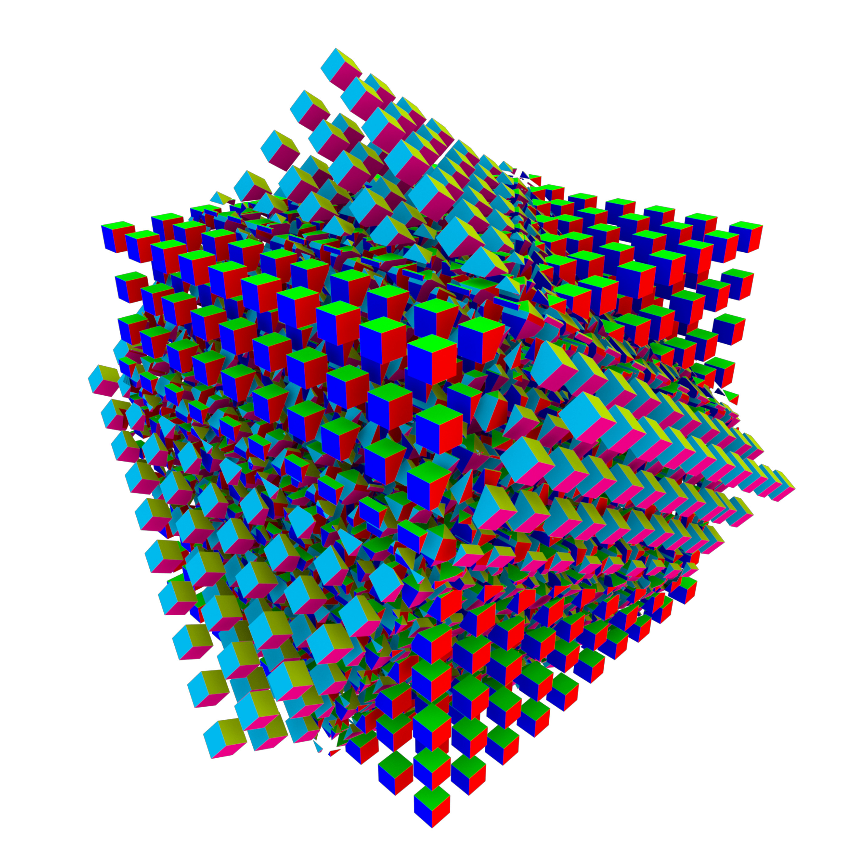
Figure 1: Arrangement of $2000=2\times10\times10\times10$ cubes

API

Every function strictly relative to the arrangement has been collected in the Lar.Arrangement sub-module but the two main functions are accessible directly from the LinearAlgebraicRepresentation namespace.

spatial_arrangement(V::Points, copEV::ChainOp, copFE::ChainOp; [multiproc::Bool])

planar_arrangement(V::Points, EV::ChainOp, [sigma::Chain], [return_edge_map::Bool], [multiproc::Bool])

Theoretical basis

The algorithm is based on the concept of recursive problem simplification (a sort of divide et impera philosophy); if we have a $d$-complex, for every ($d-1$)-cell embedded into the $\mathbb{E}^d$ euclidean space, we bring the cell, and every other cell that could intersect it, down into $\mathbb{E}^{d-1}$. We do this until we reach the $d=1$ in $\mathbb{E}^1$ case; in here, we fragment all the $1$-cells. Then, we travel back to the original $d$-dimension, and, for each dimensional step, we build correct complexes from cells provided by the fragmentation of the lower dimension.

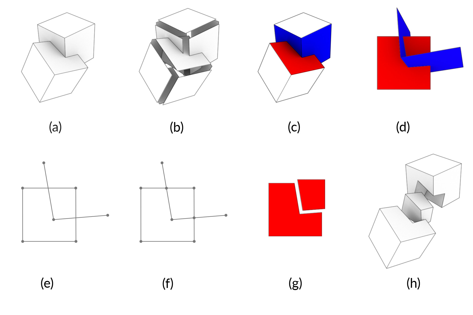
Figure 2: Algorithm overview

We have in input two cellular complexes [fig. 2, a], given as 2-skeletons, which are the sets of 2-cells [fig. 2, b, exploded]. Once we merged the skeletons, we individuate for each $2$-cell (that we will call $\sigma$) all the other cells that could intersect it. We do this by computing the spatial index: it is a mapping $\mathcal{I}(\sigma)$ from a cell $\sigma$ to every other cell $\tau$ of which $box(\sigma) \cap box(\tau) \neq \emptyset$, where the $box$ function provides the axis aligned bounding box (AABB) of a cell [fig. 2, c, $\sigma$ in red and $\mathcal{I}(\sigma)$ in blue]. The spatial arrangement calculation is speeded up by storing the AABBs as dimensional wise intervals into an interval tree \cite{intervaltrees}. Now for each cell $\sigma$ we transform $\sigma \cup \mathcal{I}(\sigma)$ in a way that $\sigma$ lays on the ``x3=0$plane [fig. 2, d] and we find the intersections of the$\mathcal{I}(\sigma)$cells with$x_3=0$plane. So we have a "soup" of 1-cells in$\mathbb{E}^2$[fig. 2, e], and we fragment each 1-cell with every other cell obtaining a valid 1-skeleton [fig. 2, f]. From this data it is possible to build the 2-cells using the ALGORITHM 1 presented and explored by Paoluzzi et al. \cite{Paoluzzi} [fig. 2, g, exploded]. The procedure to fragment 1-cells on a plane and return a 2-complex is called *planar arrangement*. When the planar arrangement is complete, fragmented$\sigma$can be transformed back to its original position in$\mathbb{E}^3``. With every 2-cell correctly fragmented, we can use the already cited ALGORITHM 1 again to build a full 3-complex [fig. 2, h, exploded]. This is possible because ALGORITHM 1 is (almost) dimension independent.

The "$1$-cells in $\mathbb{E}^2$" base case

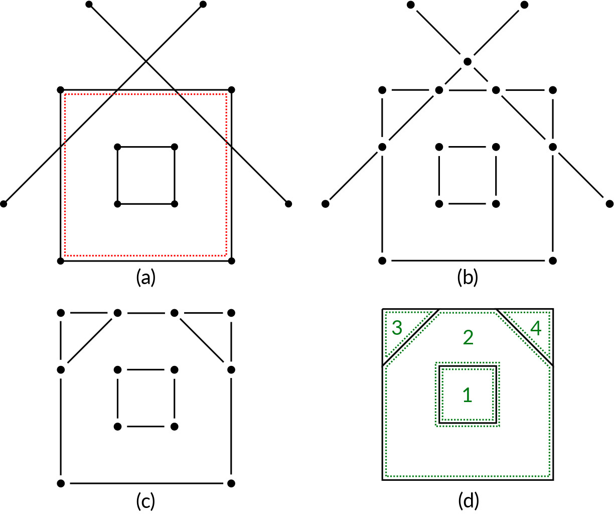
Figure 3: Planar arrangement overview

This is our base case. We have called planar arrangement the procedure to handle this case since it literally arranges a bunch of edges laying on a plane. So, in input there are 1-cells in $\mathbb{E}^2$ and, optionally (but very likely), the boundary of the original 2-cell $\sigma$ [fig. 3, a, $\sigma$ in red]. We consider each edge and we fragment it with every other edge. This brings to the creation of several coincident vertices: these will be eliminated using a KD-Tree [fig. 3, b, exploded]. At this point we have a perfectly fragmented 1-complex but many edges are superfluous and must be eliminated; two kind of edges are to discard: the ones outside the area of $\sigma$ and the ones which are not part of a maximal biconnected component (We can talk about biconnected components because we can consider the 1-skeleton as a graph: 0-cells are nodes, 1-cells are edges and the boundary operator is a incidence matrix.). The result of this edge pruning outputs a 1-skeleton [fig. 3, c, exploded].

After this, 2-cells must be computed: For each connected component we build a containment tree, which indicates which component is spatially inside an other component. Computing these relations lets us launch the ALGORITHM 1 \cite{Paoluzzi} on each component and then combine the results to create 2-cells with non-intersecting shells [fig. 3, d, 2-cells numbered in green; please note that cell 2 has cell 1 as an hole].