LAR
LAR is a general representation scheme for geometric and topological modeling (see "Linear algebraic representation for topological structures"). The domain of the scheme is provided by cellular complexes while its codomain is a set of sparse matrices. The main advantages of the scheme are:
- It is extremely effective to easily represent general non-manifold solids. For example, the memory representation of a $d=3$ cellular complex using LAR consists in only two binary sparse matrices for the topology and a bi-dimensional array for the geometry.
- Computation and analysis of cellular complexes is done only through easy linear algebra operations. The most common operation is the sparse matrix-vector multiplication.
Here a list of fundamental concepts and features of LAR:
LAR model
A LAR model is a pair geometry, topology. The geometry is specified by the position vectors of vertices in a Euclidean space $\mathbb{E}^d$ of points with $d$ coordinates. The topology is specified by one or more bases of singleton $k$-chains (i.e.~$k$-cells) for $0 \leq k\leq d$. The vertex sharing between cells implicitly provides the attachment maps between cells of various dimensions. Vertex positions are represented, by columns, by a 2-array of $d$ real coordinates.
Chains as arrays
Chain-based modeling and computing (refer to "Chain-Based Representations for Solid and Physical Modeling") is based on representation of $p$-cell subsets as chains, elements of linear spaces $C_p$ ($0\leq p\leq d$) generated by the space decomposition induced by a cellular complex, also said CW-complex. Chains can be simply represented as arrays of signed integers, one of simplest and more efficient data structure of most languages, particularly when oriented to scientific computing. Therefore, basic algebraic operations on chains as vectors (sum and product times a scalar) are implemented over arrays.
Characteristic matrices
The LAR representation scheme, i.e. our mapping between mathematical models of solids and their computer representations, uses linear chain spaces $C_p$ as models, and sparse characteristic matrices $M_p$ of $p$-cells as symbolic representations, where the $p$-cell $\sigma^k\in\Lambda_p$ is represented as the $k$-th binary row of the sparse characteristic matrix $M_p: C_0\to C_p$.
Boundary and coboundary matrices
The boundary matrix $[\partial_p]$ is the matrix of the boundary operator $\partial_p: C_p\to C_{p-1}$ ($1\leq p\leq d$) that for each chain $c_p\in C_p$ returns the boundary $(p-1)$-cycle of its $(d-1)$-faces. A boundary operator is linear: $\partial_p c + d = \partial_p c + \partial_p d$, for each $c,d\in C_p$. A cycle is a chain without boundary. Hence, the boundary of a boundary is the zero map: $partial_{p-1} \circ partial_p = 0$ ($2\leq p\leq d$).
Incidence matrices
Incidence operators between chain spaces of different dimension are easy to compute by matrix products of characteristic matrices, possibly transposed. Since both characteristic and operator matrices are very sparse, their products are computed with specialized algorithms for sparse matrices, whose complexity is roughly linear in the size of the output sparse matrix, i.e., in the number of its stored non-zero elements. Incidence queries and other types of geometric or topological computations are not performed element-wise, that necessarily require iterative or recursive programming patterns, but only require matrix product times whole chains (sets of cells), so adapting naturally to parallel and/or dataflow computational patterns found in HPC and CNN architectures.
Validity test of a representation
Data validity is easy to test by checking for satisfaction of basic equations $\partial\partial=\emptyset$ of a chain complex.
Space arrangments
Given a finite collection $\mathcal{S}$ of cellular complexes in $\mathbb{E}^d$, $d \in \{2,3\}$, the \emph{arrangement} $\mathcal{A}(\mathcal{S})$ is the decomposition of $\mathbb{E}^d$ into connected cells of dimensions $0, 1, \ldots, d$ induced by $\mathcal{S}$. In Lar.jl, we provide an efficient computation of the arrangement produced by a given set of cellular complexes in either 2D or 3D. The goal here is to provide a complete description of the plane or space decomposition induced by the input, into cells of dimensions 0, 1, 2 or 3. This computation is based on the algorithms introduced in \cite{DBLP:journals/corr/PaoluzziSD17} which describe how to compute the $d$-space arrangement generated by a collection of $(d$-$1)$-complexes. A general description of both the motivations and the features of the space arrangement and Lar.jl in general are given in~\cite{DBLP:journals/corr/abs-1710-07819}.
With abuse of language, we consider a finite cellular complex $X$ as generated by a discrete partition of an Euclidean space. In computing a cellular complex as the space arrangement of a collection of geometric objects $\mathcal{S}$, i.e. when $X := \mathcal{A}(\mathcal{S})$, we actually compute the whole chain complex $C_\bullet$ generated by $X$, i.e.:
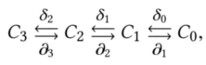
where $C_p$ ($0\geq p\geq 3$) is a linear space of \emph{$p$-chains} (subsets of $p$-cells with algebraic structure). The linear operators $\partial_p$ and $\delta_p$ are the boundary and coboundary operators as described before, respectively with
$\partial_{p-1}\circ\partial_p = \emptyset = \delta_{p}\circ\delta_{p-1},$
and where
$\delta_{p-1} = \partial_p^\top, \quad 1\leq p\leq 3$